Example of Voxel-based Analysis in SPM
The voxel-based analysis is performed in a similar way as it is done in humans. The following steps are recommended:
- Select the appropriate small animal atlas
- Perform spatial normalization of the images to the reference template
- Normalize the uptake signal
- Apply the brain mask to all the images
- Smooth the images (Implicit masking : Yes)
- Define the statistical model
- Estimate the model
- Display the results
Note: SAMIT interface must remain open during the whole procedure otherwise the default human brain parameters will be used
In this section we will go through all the steps needed to perform the data analysis using an example data set.
- Download the data set an extract its content into a new folder. The data set consist of [11C]PK11195PET brain images obtained from male Wistar rats, including a healthy group (n=13) and an intervention group with Herpes Encephalitis (HSE).
- In Matlab, go to the folder where the data set has been extracted. It is always recommended to define a working folder, since several files may be generated by SPM and located by default in the working directory.
- Start SPM by typing in Matlab:
spm pet
- From the
Toolbox menu in SPM interface select samit
- Select the small animal atlas to be used. In this example select
Schwarz - Rat
- Define the location of the ‘origin’ of coordinates. In this data set, the current location of the origin is in the center of the image. This information can be checked using the
Display option in SPM. In SAMIT interface, select bregma option in the Reorient / Fix images section, and click Reorient button. Select all the images located in the folders HSE and Healthy.
This process will relocate the origin in a position of the image close to where bregma is expected to be. The new images will be located in the same folder than the original ones but with the prefix r
- An automatic registration of the images was performed during its pre-processing. The alignment between images can be observed by selecting several images with
Check Reg in the SPM interface. Nevertheless, we are going to perform again the automatic registration process for a better alignment with the template.
- Select the
almost rigid body option in the ‘Spatial Registration’ section
- Click in
Normalise multimple images
- Select all the images from the Healthy and HSE folders
- Select the tracer-specific template ([11C]PK11195_Wistar_Template.nii) located inside the SAMIT folder. The new images will be located in the same folder than the original ones, but with the prefix w
- Normalize uptake: Information about the injected dose and the weight of the animals is provided in the file SUV table.txt
- Click on
Create table
- Select all the files created recently with the prefix wr
- Select a name for the new file that will be created
- Open the file with a text or spreadsheet editor. Fill the information according to the one provided in SUV table.txt. No data was collected for the glucose level, so there is no need for the last column and it can be removed. Save the file as tabulated text file or as Excel file
- Select the image units. In this study, the original images were acquired in Bq/cc
- Select the normalization procedure. For this example we will use the SUV (default) option
- Click in
Create normalized images. The new images will be located in the same folder than the previous ones, but including the suffix -SUV
- Apply a mask to the whole brain. This step will avoid the influence of uptake outside the brain during the smoothing procedure, and it will avoid errors if global normalization is used during the statistical model
- Click in the
Brain Mask button
- Select the images to which apply the mask (i.e. those with the suffix –SUV)
- The new images will be located in the same folder than the previous ones with the prefix m
- Apply smoothing to the image:
- Click in
Smooth button from the SPM interface
- Select the images to smooth (i.e. those with the prefix m)
- Select the desired FWHM. For this example we can leave the default value of 1.2 mm (i.e. recommend values are between 0.8 and 0.12 mm for rat studies)
- Select Implicit masking to Yes. This will avoid the smoothing to go outside the masked region
- Run the batch: Click on the icon of a green arrow or select
File > Run Batch
- The new images will be located in the same folder than the previous ones with the prefix s. These are the final images to be used in the voxel-based analysis
- Basic model: First we have to define the statistical model. In the present example it is a simple two-sample t-test design (for further details, please refer to the SPM manual)
- Click on
Basic Models button in the main SPM window
- Directory: choose the directory were data will be written (e.g. workspace)
- Select the Design as Two-sample t-test
- Select the Healthy group as Group 1 scans
- Select the HSE group as Group 2 scans
- Select Explicit Mask, using the whole brain mask located in SAMIT folder (i.e. Schwarz_intracranialMask.nii)
- Estimate the model
- In the menu of the Batch Editor select
SPM > Stats > Model estimation
- Select the new module
Model estimation from the left section of the Batch Editor
- Click on
Dependency button, located in the lower right section
- Select the Factorial design option
- Save the batch for future modifications
- Run the batch: Click on the icon of a green arrow or select
File > Run Batch
- Show the results
- Click on
Results button in the main SPM window
- Select the SPM.mat file located in the directory selected previously during the especification of the model
- Click on
Define a new contrast 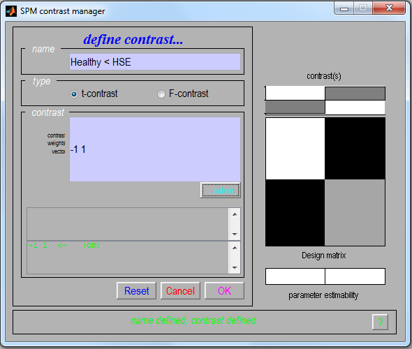
- In the name type Healthy < HSE
- Select: t-contrast
- Contrast: -1 1
- Click on
OK
- Select the contrast and press
Done
- Apply masking:
none
- Title for comparison: leave the current title and press enter
- Choose the p value adjustment (FWE or uncorrected). In this example select
none
- Choose the p value. In this example type: 0.001
- Extent threshold (voxels). In this example type: 0
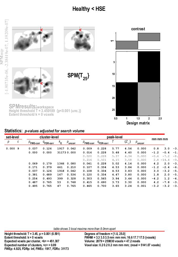
- We will explore the results in a “two-steps” approach, using an uncorrected p-threshold at voxel level, and a FWE corrected threshold at cluster level.
- Look a the botom of the results section for the value asigned to FWEc:, in this case 1917
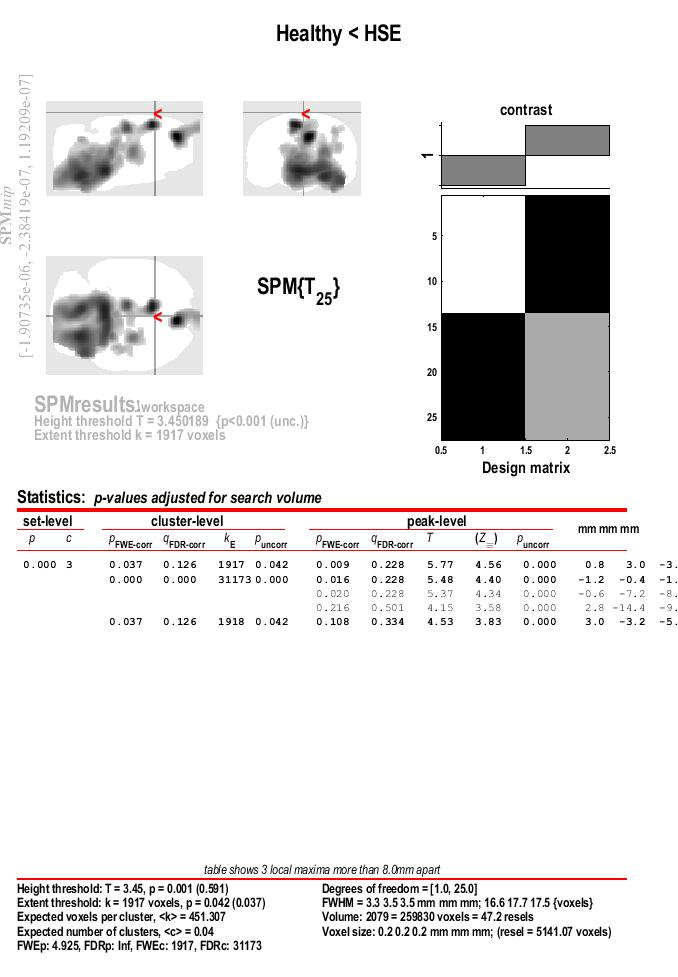
- Run the results again, clicl on
Contrast > Significance level > Change ... , witht the same settings as before for the “p value adjustment” and the “ p value” itself
- Choose the p value adjustment (FWE or uncorrected). Like before, select
none
- Choose the p value. Like before, type: 0.001
- Extent threshold (voxels). At this second step, use the value of the FWE,, in this example 1917
- Results are presented in a maximum intensity projection (MIP) display on a glass rat brain. Since the MRI rat template was spatially aligned with the Paxinos atlas the resulting coordinates are equivalent to those in the atlas. In addition, with only those cluster found to be statistically significant after FWE correction are displayed.
- To visualize the results over the MRI go to
Display > Overlays… > Section and choose the rat MRI template located in the SAMIT folder
 The aim of this toolbox is to facilitate voxel-based and/or volume-based analysis of small animal PET and SPECT brain images. It also provides an automatized procedure for the construction of new tracer-specific templates for the spatial registration of small animal PET and SPECT brain images.